Hypothesis Testing

A statistical hypothesis is an assumption about a population parameter. This assumption may or may not be true. Hypothesis testing refers to the formal procedures used by statisticians to accept or reject statistical hypotheses. The null hypothesis is essentially the "devil's advocate" position. That is, it assumes that whatever you are trying to prove did not happen. The null hypothesis is initially assumed to be true.

• Null Hypothesis - the hypothesis that sample observations result purely from chance
• Alternate Hypothesis - the hypothesis that sample observations are influenced by some non-random cause

Decision Errors

• Type I error - Rejects a null hypothesis when it is true. The probability of committing a Type I error is called the significance level. This probability is also called alpha, and is often denoted by $\alpha$.
• Type II error - Fails to reject a null hypothesis that is false. The probability of committing a Type II error is called Beta, and is often denoted by $\beta$. The probability of not committing a Type II error is called the Power of the test.

Decision Rules

• P-value - The strength of evidence in support of a null hypothesis is measured by the P-value. The P-value is the probability of observing a test statistic as extreme as the test statistic, assuming the null hypotheis is true. If the P-value is less than the significance level, we reject the null hypothesis.

  The P-value approach involves determining "likely" or "unlikely" by determining the probability — assuming the null hypothesis were true — of observing a more extreme test statistic in the direction of the alternative hypothesis than the one observed.

  1. Specify null and alternate hypothesis

  2. Calculate test statistic

  3. Determine p-value. "If the null hypothesis is true, what is the probability of observing a more extreme test statistic in the direction of the alternative hypothesis?"

  4. Compare p-value to $\alpha$

  | Right Tailed | Left Tailed | Two Tailed | | :--- | :--- | :--- | | 1 - stats.t.cdf(x=2.5, df=14, loc=0, scale=1) | stats.t.cdf(x=2.5, df=14, loc=0, scale=1) | stats.t.cdf(x=2.5, df=14, loc=0, scale=1) * 2 |

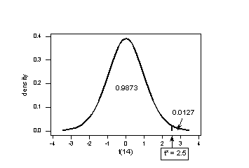
The P-value for conducting the two-tailed test $H_0 : \mu = 3$ versus $H_1 : \mu \ne 3$ is the probability that we would observe a test statistic less than -2.5 or greater than 2.5 if the population mean $\mu$ really were 3. The P-value for a two-tailed test is always two times the P-value for either of the one-tailed tests. The P-value, 0.0254, tells us it is "unlikely" that we would observe such an extreme test statistic in the direction of $H_1$ if the null hypothesis is true. Therefore, our initial assumption that the null hypothesis is true must be incorrect. That is, since the P-value, 0.0254, is less than $\alpha$ = 0.05, we reject the null hypothesis.

The P-value is the probability of how extreme is $H_1$. If P-value is high, $H_1$ is very extreme and is unlikely to happen and thus accept null as there is not sufficient evident. If P-value is low, $H_1$, is not very extreme and is likely to happen and thus reject null as there is sufficient evidence.

• Region of acceptance - If the test statistic falls within the region of acceptance, the null hypothesis is not rejected. The region of acceptance is defined so that the chance of making a Type I error is equal to the significance level. The set of values outside the region of acceptance is called the region of rejection. If the test statistic falls within the region of rejection, the null hypothesis is rejected.

  If the test statistic is more extreme than the critical value, then the null hypothesis is rejected in favor of the alternative hypothesis. If the test statistic is not as extreme as the critical value, then the null hypothesis is not rejected.

  1. Specify null and alternate hypothesis

  2. Calculate test statistic

  3. Determine the critical value by finding the value of the known distribution of the test statistic such that the probability of making a Type I error is equal to the specified significant level

  4. Compare test statistic to critical value

  | Right Tailed | Left Tailed | Two Tailed | | :--- | :--- | :--- | | t (0.05, 14)stats.t.ppf(q=1-0.05, df=14, loc=0, scale=1) | - t(0.05, 14)stats.t.ppf(q=0.05, df=14, loc=0, scale=1) | t (0.05/2, 14)stats.t.ppf(q=0.05/2, df=14, loc=0, scale=1), stats.t.ppf(q=1-(0.05/2), df=14, loc=0, scale=1) |

One-Tailed and Two-Tailed Tests

A test of a statistical hypothesis, where the region of rejection is on only one side of the sampling distribution, is called a one-tailed test. For example, suppose the null hypothesis states that the mean is less than or equal to 10. The alternative hypothesis would be that the mean is greater than 10. The region of rejection would consist of a range of numbers located on the right side of sampling distribution; that is, a set of numbers greater than 10.

A test of a statistical hypothesis, where the region of rejection is on both sides of the sampling distribution, is called a two-tailed test. For example, suppose the null hypothesis states that the mean is equal to 10. The alternative hypothesis would be that the mean is less than 10 or greater than 10. The region of rejection would consist of a range of numbers located on both sides of sampling distribution; that is, the region of rejection would consist partly of numbers that were less than 10 and partly of numbers that were greater than 10.

Power of a Hypothesis Test

The probability of not committing a Type II error is called the power of a hypothesis test.

Effect Size

To compute the power of the test, one offers an alternative view about the "true" value of the population parameter, assuming that the null hypothesis is false. The effect size is the difference between the true value and the value specified in the null hypothesis.

Effect size = True value - Hypothesized value

For example, suppose the null hypothesis states that a population mean is equal to 100. A researcher might ask: What is the probability of rejecting the null hypothesis if the true population mean is equal to 90? In this example, the effect size would be 90 - 100, which equals -10.

Factors That Affect Power

The power of a hypothesis test is affected by three factors.

• Sample size (n). Other things being equal, the greater the sample size, the greater the power of the test.

• Significance level ($\alpha$). The higher the significance level, the higher the power of the test. If you increase the significance level, you reduce the region of acceptance. As a result, you are more likely to reject the null hypothesis. This means you are less likely to accept the null hypothesis when it is false; i.e., less likely to make a Type II error. Hence, the power of the test is increased.

• The "true" value of the parameter being tested. The greater the difference between the "true" value of a parameter and the value specified in the null hypothesis, the greater the power of the test. That is, the greater the effect size, the greater the power of the test.

Hypothesis Test: Proportions (one sample t-test)

• Standard Deviation = $\sigma =$
• Test Statistic: z-score

Example 1:

The CEO of a large electric utility claims that 80 percent of his 1,000,000 customers are very satisfied with the service they receive. To test this claim, the local newspaper surveyed 100 customers, using simple random sampling. Among the sampled customers, 73 percent say they are very satisified. Based on these findings, can we reject the CEO's hypothesis that 80% of the customers are very satisfied? Use a 0.05 level of significance.

Example 2:

Suppose the previous example is stated a little bit differently. Suppose the CEO claims that at least 80 percent of the company's 1,000,000 customers are very satisfied. Again, 100 customers are surveyed using simple random sampling. The result: 73 percent are very satisfied. Based on these results, should we accept or reject the CEO's hypothesis? Assume a significance level of 0.05.

Hypothesis Test: Difference between Proportions (two sample t-test)

• Standard Error :
• Test Statistic :

Example 1:

Suppose the Acme Drug Company develops a new drug, designed to prevent colds. The company states that the drug is equally effective for men and women. To test this claim, they choose a a simple random sample of 100 women and 200 men from a population of 100,000 volunteers. At the end of the study, 38% of the women caught a cold; and 51% of the men caught a cold. Based on these findings, can we reject the company's claim that the drug is equally effective for men and women? Use a 0.05 level of significance.

Example 2:

Suppose the previous example is stated a little bit differently. Suppose the Acme Drug Company develops a new drug, designed to prevent colds. The company states that the drug is more effective for women than for men. To test this claim, they choose a a simple random sample of 100 women and 200 men from a population of 100,000 volunteers. At the end of the study, 38% of the women caught a cold; and 51% of the men caught a cold. Based on these findings, can we conclude that the drug is more effective for women than for men? Use a 0.01 level of significance.

Hypothesis Test: Mean (one sample t-test)

• Standard Error :
• Test Statistic : t-statistic

Example 1:

An inventor has developed a new, energy-efficient lawn mower engine. He claims that the engine will run continuously for 5 hours (300 minutes) on a single gallon of regular gasoline. From his stock of 2000 engines, the inventor selects a simple random sample of 50 engines for testing. The engines run for an average of 295 minutes, with a standard deviation of 20 minutes. Test the null hypothesis that the mean run time is 300 minutes against the alternative hypothesis that the mean run time is not 300 minutes. Use a 0.05 level of significance. (Assume that run times for the population of engines are normally distributed.)

Example 2:

Bon Air Elementary School has 1000 students. The principal of the school thinks that the average IQ of students at Bon Air is at least 110. To prove her point, she administers an IQ test to 20 randomly selected students. Among the sampled students, the average IQ is 108 with a standard deviation of 10. Based on these results, should the principal accept or reject her original hypothesis? Assume a significance level of 0.01. (Assume that test scores in the population of engines are normally distributed.)

Hypothesis Test: Difference between Means (two sample t-test)

• Standard Error :
• Test Statistic : t-statistic

Example 1:

Within a school district, students were randomly assigned to one of two Math teachers - Mrs. Smith and Mrs. Jones. After the assignment, Mrs. Smith had 30 students, and Mrs. Jones had 25 students. At the end of the year, each class took the same standardized test. Mrs. Smith's students had an average test score of 78, with a standard deviation of 10; and Mrs. Jones' students had an average test score of 85, with a standard deviation of 15. Test the hypothesis that Mrs. Smith and Mrs. Jones are equally effective teachers. Use a 0.10 level of significance. (Assume that student performance is approximately normal.)

Example 2:

The Acme Company has developed a new battery. The engineer in charge claims that the new battery will operate continuously for at least 7 minutes longer than the old battery. To test the claim, the company selects a simple random sample of 100 new batteries and 100 old batteries. The old batteries run continuously for 190 minutes with a standard deviation of 20 minutes; the new batteries, 200 minutes with a standard deviation of 40 minutes. Test the engineer's claim that the new batteries run at least 7 minutes longer than the old. Use a 0.05 level of significance. (Assume that there are no outliers in either sample.)

Hypothesis Test: Difference between Pairs

Hypothesis Test: Chi-Square Goodness of Fit

The test is applied when you have one categorical variable from a single population. It is used to determine whether sample data are consistent with a hypothesized distribution.

$H_0$: The data are consistent with a specified distribution

$H_1$: The data are not consistent with a specified distribution

• Degree of Freedom : Number of levels of the categorical variable minus 1
• Test Statistic : Chi Square statistic

Example 1:

Acme Toy Company prints baseball cards. The company claims that 30% of the cards are rookies, 60% veterans, and 10% are All-Stars. Suppose a random sample of 100 cards has 50 rookies, 45 veterans, and 5 All-Stars. Is this consistent with Acme's claim? Use a 0.05 level of significance.

Hypothesis Test: Chi-Square Test of Homogenity

The test is applied to a single categorical variable from two or more different populations. It is used to determine whether frequency counts are distributed identically across different populations.

• Degree of Freedom : (r - 1) * (c - 1), where r is the number of populations, and c is the number of levels for the categorical variable
• Test Statistic : Chi Square statistic

Example 1:

In a study of the television viewing habits of children, a developmental psychologist selects a random sample of 300 first graders - 100 boys and 200 girls. Each child is asked which of the following TV programs they like best: The Lone Ranger, Sesame Street, or The Simpsons. Results are shown in the contingency table below.

Viewing Preferences Row total

Lone Ranger Sesame Street The Simpsons

Boys 50 30 20 100

Girls 50 80 70 200

Column total 100 110 90 300

Do the boys' preferences for these TV programs differ significantly from the girls' preferences? Use a 0.05 level of significance.

Hypothesis Test: Chi-Square Test of Independence

The test is applied when you have two categorical variables from a single population. It is used to determine whether there is a significant association between the two variables.

$H_0$: Variable A and Variable B are independent

$H_1$: Variable A and Variable B are not independent

• Degree of Freedom : (r - 1) * (c - 1), where r is the number of populations, and c is the number of levels for the categorical variable
• Test Statistic : Chi Square statistic

Example 1:

A public opinion poll surveyed a simple random sample of 1000 voters. Respondents were classified by gender (male or female) and by voting preference (Republican, Democrat, or Independent). Results are shown in the contingency table below.

Voting Preferences Row total

Republican Democrat Independent

Male 200 150 50 400

Female 250 300 50 600

Column total 450 450 100 1000

Is there a gender gap? Do the men's voting preferences differ significantly from the women's preferences? Use a 0.05 level of significance.

Hypothesis Test: Regression Slope

This test determines whether there is a significant linear relationship between an independent variable X and a dependent variable Y. The test focuses on the slope of the regression line. If we find that the slope of the regression line is significantly different from zero, we will conclude that there is a significant relationship between the independent and dependent variables.

$H_0$: $\beta_1 = 0$

$H_1$: $\beta_1 \ne 0$

If there is a significant linear relationship between the independent variable X and the dependent variable Y, the slope will not equal zero. The null hypothesis states that the slope is equal to zero, and the alternative hypothesis states that the slope is not equal to zero.

Confidence Interval for $\beta_1$, sample estimate +- (t-multiplier x standard error)

$\beta_1 \pm t_{(\alpha/2, n-2)}\times \left( \frac{\sqrt{MSE}}{\sqrt{\sum(x_i-\bar{x})^2}} \right)$ The resulting confidence interval not only gives us a range of values that is likely to contain the true unknown value $\beta_1$. It also allows us to answer the research question "is the predictor x linearly related to the response y?" If the confidence interval for $\beta_1$ contains 0, then we conclude that there is no evidence of a linear relationship between the predictor x and the response y in the population. On the other hand, if the confidence interval for $\beta_1$ does not contain 0, then we conclude that there is evidence of a linear relationship between the predictor x and the response y in the population.

$t^*=\frac{\beta_1-\beta}{\left(\frac{\sqrt{MSE}}{\sqrt{\sum(x_i-\bar{x})^2}} \right)}=\frac{\beta_1-\beta}{se(\beta_1)}$